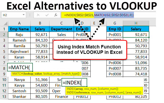
Some Known Facts About How To Do Vlookup.

Use VLOOKUP when you need to locate things in a table or a variety by row. For example, seek out a rate of an auto component by the part number, or find an employee name based upon their employee ID. In its simplest form, the VLOOKUP feature says: =VLOOKUP(What you desire to search for, where you intend to look for it, the column number in the range containing the worth to return, return an Approximate or Precise suit-- showed as 1/TRUE, or 0/FALSE).

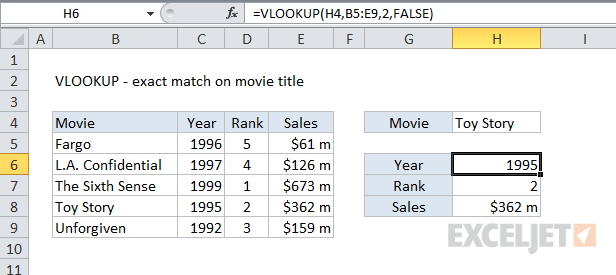
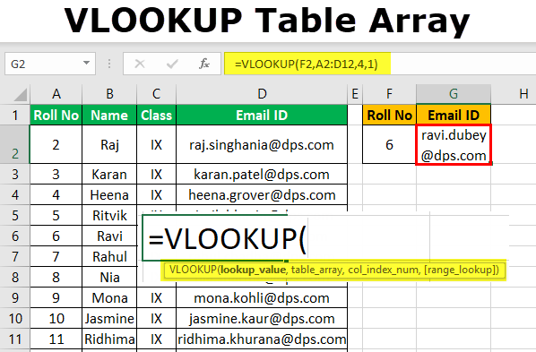
Make use of the VLOOKUP function to seek out a worth in a table. Phrase structure VLOOKUP (lookup_value, table_array, col_index_num, [range_lookup] For instance: =VLOOKUP(A 2, A 10: C 20,2, TRUE) =VLOOKUP("Fontana", B 2: E 7,2, FALSE) =VLOOKUP(A 2,'Client Details'! A: F,3, FALSE) Argument name Description lookup_value (required) The value you want to seek out. The worth you desire to look up must remain in the very first column of the range of cells you define in the table_array disagreement.

Lookup_value can be a value or a recommendation to a cell. table_array (required) The series of cells in which the VLOOKUP will look for the lookup_value and the return value. You can make use of a called variety or a table, as well as you can use names in the disagreement as opposed to cell references.

The cell array additionally requires to consist of the return worth you intend to locate. Discover how to pick ranges in a worksheet. col_index_num (called for) The column number (beginning with 1 for the left-most column of table_array) that has the return worth. range_lookup (optional) A logical value that specifies whether you desire VLOOKUP to discover an approximate or a specific match: Approximate suit - 1/TRUE thinks the very first column in the table is arranged either numerically or alphabetically, as well as will certainly after that look for the closest value.

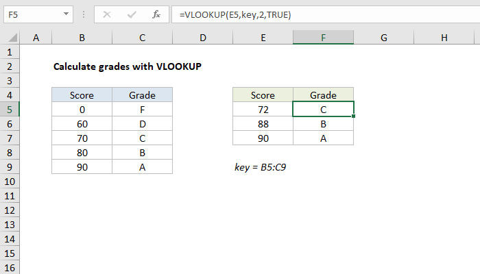
For instance, =VLOOKUP(90, A 1: B 100,2, REAL). Precise suit - 0/FALSE look for the specific value in the first column. As an example, =VLOOKUP("Smith", A 1: B 100,2, FALSE). There are four pieces of information that you will require in order to construct the VLOOKUP syntax: The worth you desire to search for, also called the lookup value.

The Definitive Guide for What Is Vlookup In Excel

Keep in mind that the lookup value need to constantly be in the first column in the variety for VLOOKUP to function appropriately. For instance, if your lookup worth remains in cell C 2 then your array must start with C. The column number in the range that consists of the return value. For example, if you specify B 2:D 11 as the range, you must count B as the very first column, C as the 2nd, and so forth.

If you don't specify anything, the default worth will constantly be REAL or approximate suit. Currently put every one of the above together as complies with: =VLOOKUP(lookup worth, range containing the lookup value, the column number in the variety having the return worth, Approximate match (REAL) or Exact suit (FALSE)). Below are a few instances of VLOOKUP: Trouble What failed Incorrect value returned If range_lookup is TRUE or neglected, the first column requires to be arranged alphabetically or numerically.

Either sort the very first column, or utilize FALSE for a precise match. #N/ A in cell If range_lookup holds true, after that if the value in the lookup_value is smaller sized than the smallest value in the first column of the table_array, you'll get the #N/ A mistake value. If range_lookup is FALSE, the #N/ An error worth indicates that the specific number isn't discovered.

#REF! in cell If col_index_num is more than the number of columns in table-array, you'll get the #REF! mistake worth. To learn more on dealing with #REF! errors in VLOOKUP, see Just how to fix a #REF! mistake. #VALUE! in cell If the table_array is less than 1, you'll get the #VALUE! error worth.

#NAME? in cell The #NAME? error worth generally implies that the formula is missing out on quotes. To seek out a person's name, make certain you make use of quotes around the name in the formula. For example, get in the name as "Fontana" in =VLOOKUP("Fontana", B 2: E 7,2, FALSE). For more details, see Just how to correct a #NAME! mistake.

Vlookup Example Can Be Fun For Everyone

Discover exactly how to make use of outright cell referrals. Don't store number or day values as message. When looking number or day values, be certain the information in the very first column of table_array isn't kept as message values. Or else, VLOOKUP might return a wrong or unforeseen worth. Sort the initial column Sort the very first column of the table_array prior to making use of VLOOKUP when range_lookup is TRUE.

A question mark matches any single personality. An asterisk matches any type of series of characters. If you wish to discover a real enigma or asterisk, kind a tilde (~) before the personality. For example, =VLOOKUP("Fontan?", B 2: E 7,2, FALSE) will browse for all circumstances of Fontana with a last letter that might vary.

When browsing text worths in the initial column, make sure the information in the very first column doesn't have leading areas, routing rooms, inconsistent use straight (' or") as well as curly (' or ") quote marks, or nonprinting personalities. In these situations, VLOOKUP may return an unexpected worth.

You can always ask a professional in the Excel Individual Voice. Quick Referral Card: VLOOKUP refresher Quick Reference Card: VLOOKUP troubleshooting pointers You Tube: VLOOKUP video clips from Excel community experts Whatever you require to find out about VLOOKUP How to correct a #VALUE! error in the VLOOKUP function How to remedy a #N/ A mistake in the VLOOKUP function Summary of formulas in Excel Just how to avoid busted formulas Detect errors in formulas Excel functions (alphabetical) Excel features (by classification) VLOOKUP (totally free sneak peek).

To compute delivery cost based upon weight, you can use the VLOOKUP feature. In the example shown, the formula in F 8 is: =VLOOKUP(F 7, B 6: C 10,2,1)* F 7 This formula uses the weight to discover the right "price per kg" after that ... To override output from VLOOKUP, you can nest VLOOKUP in the IF function.

excel vlookup error handling vlookup in excel using two columns excel vlookup year